Traveling Salesman Problem and Hamiltonian Cycle

Chinese | English

This chapter introduces two classic problems in computational complexity theory:

• Hamiltonian Cycle (HC)

• Traveling Salesman Problem (TSP)

They have three important implications:

1. Both are representative NP-Complete / NP-Hard problems.

2. Both are very "intuitive," but fundamentally extremely difficult.

3. They serve as the theoretical foundation and starting point for subsequent approximation algorithms.

• Traveling Salesman Problem and Hamiltonian Cycle

  • Hamiltonian Cycle

    • Problem Definition

    • Decision Version of the HC Problem

    • Proving Hamiltonian Cycle ∈ NP

    • Hamiltonian Cycle is NP-Complete

  • Traveling Salesman Problem (TSP)

    • Problem Definition (Optimization Version vs. Decision Version)

    • Proof that TSP ∈ NP

    • TSP is NP-Complete

  • Metric TSP and Approximation Algorithms

    • Triangle Inequality

    • 2-Approximation based on MST

  • Why General TSP does not have a constant approximation

Hamiltonian Cycle

Problem Definition

Given an undirected graph $G=(V,E)$$G = (V, E)$. A Hamiltonian Cycle (HC) is a simple cycle that visits each vertex exactly once and returns to the starting point.

Decision Version of the HC Problem

We focus on the decision problem: Hamiltonian Cycle Problem

Given graph G, does a Hamiltonian Cycle exist? **

This is a standard YES/NO question, preparing for the subsequent discussion on NP-completeness.

Proving Hamiltonian Cycle ∈ NP

This problem is quite simple; proving membership in NP is usually not difficult.

Certificate: If a Hamiltonian Cycle exists in the graph, the certificate can be a sequence of vertices $v_1,v_2,\dots ,v_n$$v_1, v_2, \dots, v_n$.

Certifier: Check the following:

1. Does the sequence contain all vertices without repetition?

2. For any adjacent pair $(v_i,v_{i+1})$$(v_i, v_{i+1})$, does an edge exist?

3. Does an edge exist between $(v_n,v_1)$$(v_n, v_1)$?

These checks can all be completed in polynomial time.

Hamiltonian Cycle is NP-Complete

This is a core conclusion, and the construction in this part is quite complex.

We choose to use the Vertex Cover problem for reduction.

$\text{Vertex Cover}\le ₚ\text{Hamiltonian Cycle}$$\text{Vertex Cover} ≤ₚ \text{Hamiltonian Cycle}$

Vertex Cover:

Given a graph $G=(V,E)$$G=(V,E)$ and an integer $k$$k$, does there exist a set of vertices of size $\le k$$≤ k$ such that every edge has at least one endpoint in the set?

The core idea of ​​the reduction is:

• Transforming the choice of "selecting vertices to cover edges"

• into "the Hamiltonian Cycle must pass through the gadget in a certain way"

In other words: Does a Hamiltonian Cycle exist ⇔ Does a valid Vertex Cover exist?

The lecture slides (570) use a set of complex gadgets; we won't copy them verbatim here, but explain why this design is effective. ||| |---|---|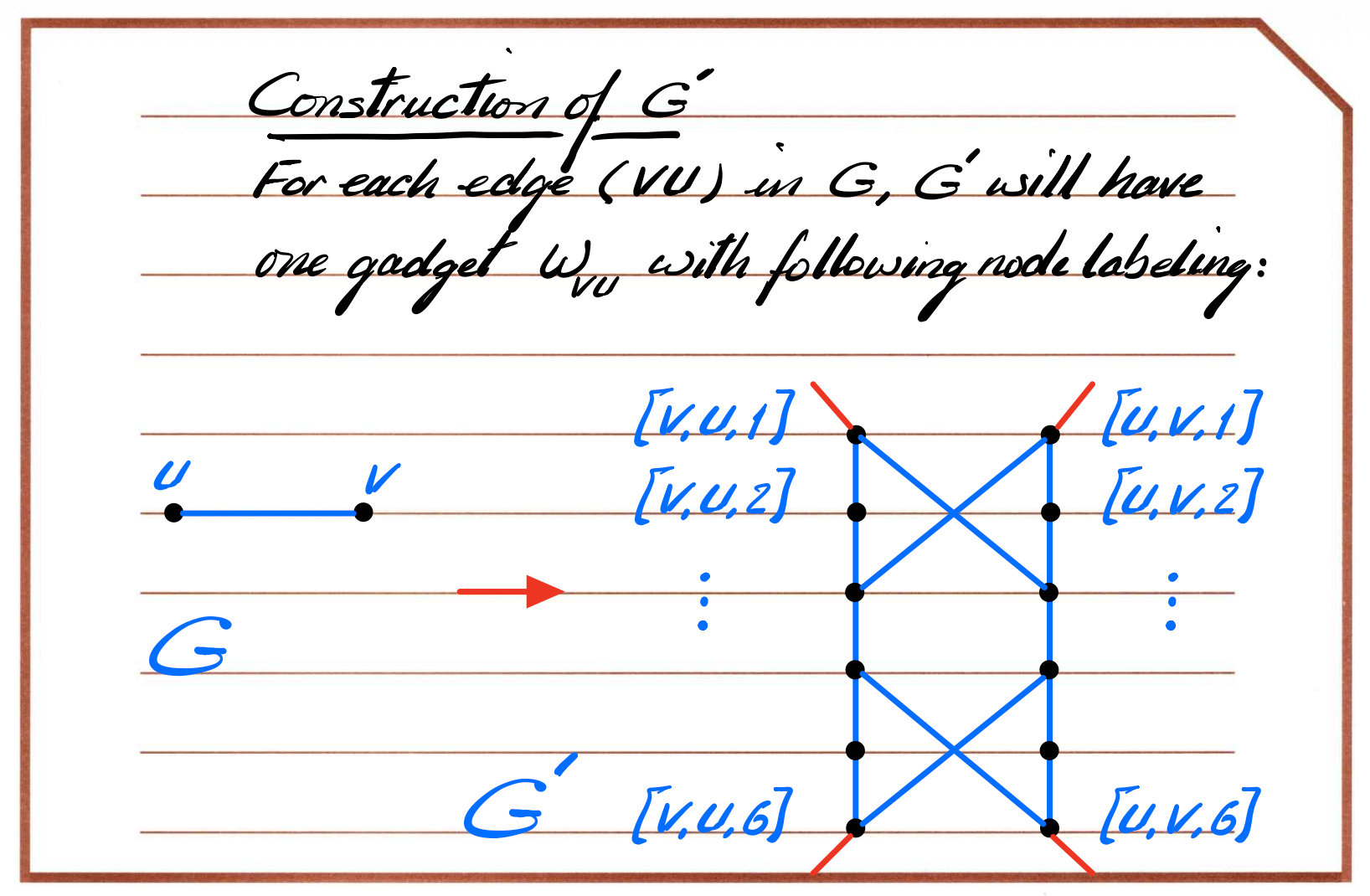

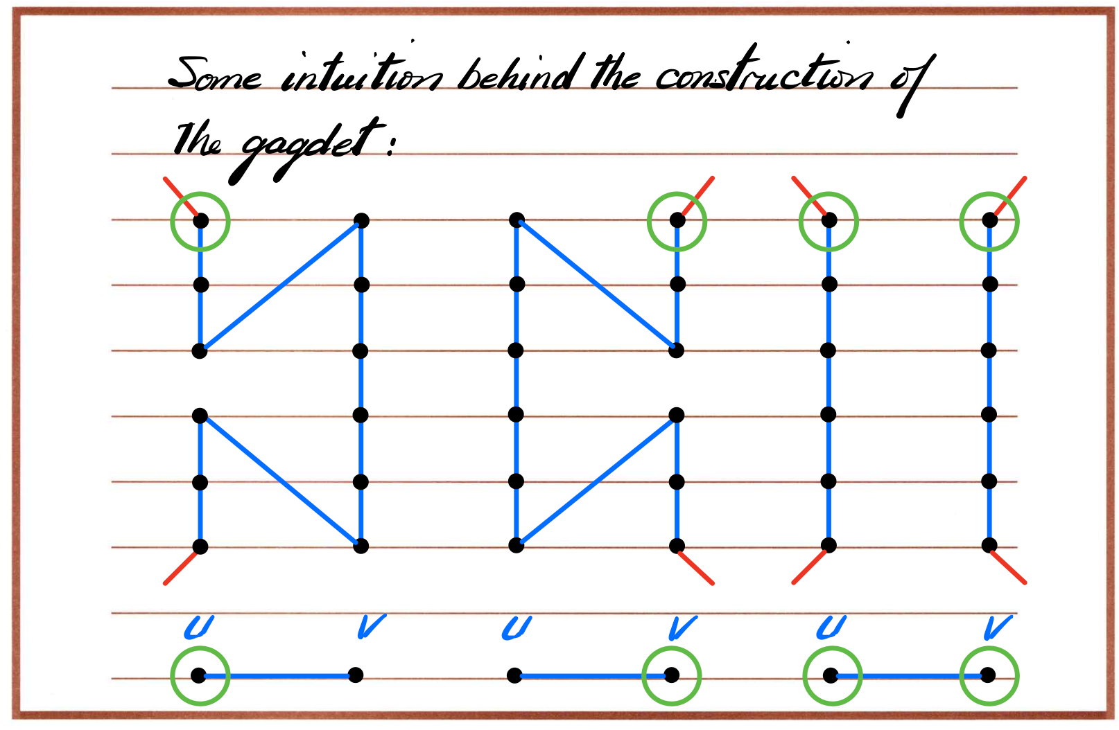
The intuition can be summarized in three points:

1. Each edge corresponds to a structure: The way the Hamiltonian Cycle passes through this structure is equivalent to "which endpoint is chosen to cover this edge."

2. Vertex selection is restricted: Through selector vertices, it is enforced that at most k "covering decisions" can be made.

3. The Hamiltonian Cycle must cover all gadgets: No gadget can be skipped, otherwise a complete cycle cannot be formed.

Therefore:

• If a vertex cover of size ≤ k exists → a Hamiltonian Cycle can be constructed.

• If a Hamiltonian Cycle exists → a vertex cover can be deduced.

Conclusion: Hamiltonian Cycle is NP-Complete

Traveling Salesman Problem (TSP)

Problem Definition (Optimization Version vs. Decision Version)

Optimization version of TSP:

Find the shortest path that visits every city once and returns to the starting point.

However, the NP-completeness discussion only concerns the decision version:

TSP (Decision Version) Given a weighted complete graph and a threshold D, does there exist a tour whose total weight is ≤ D?

Proof that TSP ∈ NP

Certificate: A permutation of cities (tour)

Certifier:

• Check if every city is visited once

• Calculate the total path length and check if it is ≤ D

All steps can be completed in polynomial time.

Therefore: TSP ∈ NP

This is all very simple.

TSP is NP-Complete

The lecture slides from course 570 use a very classic and elegant construction. Given a graph $G=(V,E)$$G=(V,E)$, construct a complete graph $G^{\prime }$$G'$:

• If $(u,v)\in E$$(u,v) \in E$, then $w(u,v)=1$$w(u,v) = 1$

• If $(u,v)\notin E$$(u,v) \notin E$, then $w(u,v)=2$$w(u,v) = 2$

And set the threshold: $D=|V|$$D = |V|$

At this point:

If the original graph has a Hamiltonian Cycle → the total cost of this cycle in the new graph = |V| → TSP answers YES

If there is no Hamiltonian Cycle → any tour contains at least one edge with weight 2 → total weight > |V| → TSP answers NO

Therefore:

Hamiltonian Cycle ≤ₚ TSP

So TSP is NP-Complete

Metric TSP and Approximation Algorithms

Triangle Inequality

Metric TSP requires edge weights to satisfy the triangle inequality:

$w(u,v)\le w(u,x)+w(x,v)$$w(u,v) \le w(u,x) + w(x,v)$

This fundamentally changes the problem structure.

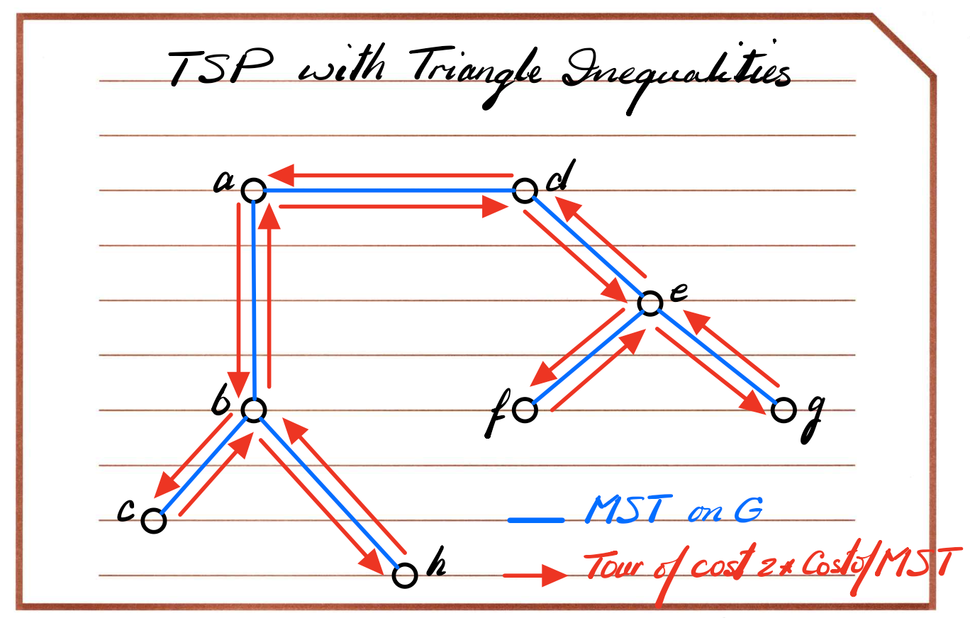
2-Approximation based on MST

The algorithm idea in the lecture slides:

1. Calculate the Minimum Spanning Tree (MST)

2. Perform a preorder traversal of the MST

3. Use the triangle inequality shortcut to handle repeated nodes

Conclusion: Metric TSP has a 2-approximation algorithm

Why General TSP does not have a constant approximation

The key conclusion is:

If General TSP has a constant approximation algorithm ⇒ Hamiltonian Cycle can be solved in polynomial time ⇒ implies P = NP

Therefore:

General TSP does not have any constant factor approximation algorithm (unless P=NP)

And this is the essential difference between Metric TSP and General TSP.